何かあれば GitHub のリポジトリに issue を作るか ryukau@gmail.com までお気軽にどうぞ。
Update: 2025-01-07
Nam, Pekonen, Valimaki による Perceptually informed synthesis of bandlimited classical waveforms using integrated polynomial interpolation で紹介されている B-spline PolyBLEP residual の 4, 6, 8 点の式を掲載します。 4 点の式は Nam の論文に掲載されている式と同じです (Table VII.) 。
式の導出の手順は PolyBLAMP Residual にまとめています。ステップ関数とランプ関数の関係と同じように、 PolyBLEP を 1 階積分すると PolyBLAMP になります。
Maxima のコードは PolyBLAMP residual で紹介したコードとほとんど同じです。変更した箇所にコメントをつけています。
N(i, k, t) :=
  if k = 1 then
    if concat('t, i) <= t and t < concat('t, i + 1) then 1 else 0
  else block([t_i: concat('t, i), t_ik: concat('t, i + k)],
    (t - t_i) / (concat('t, i + k - 1) - t_i) * N(i, k - 1, t)
    + (t_ik - t) / (t_ik - concat('t, i + 1)) * N(i + 1, k - 1, t)
  );

uniformBspline(k) := block(
  [
    result: [],
    T: makelist(concat('t, j) = j - k + 1, j, 0, 3 * k - 2)
  ],
  assume(concat('t, k - 1) <= t, t < concat('t, k)),
  for i: 0 thru 3 * k - 2 do assume(concat('t, i) < concat('t, i + 1)),
  for i: 0 thru k - 1 do
    result: endcons(expand(subst(T, N(i, k, t))), result),
  forget(concat('t, k - 1) <= t, t < concat('t, k)),
  result
);

findConstant(eq, residual) := block([result: [], J, C],
  J: integrate(last(eq), t),
  result: cons(J, result),
  C: subst(1, t, J),
  for i: length(eq) - 1 step -1 thru 1 do (
    J: integrate(eq[i], t) + C,
    C: subst(1, t, J), /* C に代入するタイミングを変更。 */
    if residual and i < length(eq) / 2 + 1 then J: J - 1, /* J - t から J - 1 に変更。 */
    result: cons(J, result)
  ),
  result
);

eq: uniformBspline(4);      /* k - 1 が次数。 */
P: findConstant(eq, false); /* 1 回積分した式。 */
R: findConstant(eq, true);  /* PolyBLEP residual */
4, 6, 8 Point の PolyBLEP residual を求めました。数式と、 wxMaxima
の Copy for Octave/Matlab
でコピーしたテキスト形式の式を掲載しています。
\[ \begin{aligned} J B_{4,0}(t) &= -\frac{{{t}^{4}}}{24}+\frac{{{t}^{3}}}{6}-\frac{{{t}^{2}}}{4}+\frac{t}{6}-\frac{1}{24}\\ J B_{4,1}(t) &= \frac{{{t}^{4}}}{8}-\frac{{{t}^{3}}}{3}+\frac{2 t}{3}-\frac{1}{2}\\ J B_{4,2}(t) &= -\frac{{{t}^{4}}}{8}+\frac{{{t}^{3}}}{6}+\frac{{{t}^{2}}}{4}+\frac{t}{6}+\frac{1}{24}\\ J B_{4,3}(t) &= \frac{{{t}^{4}}}{24}\\ \end{aligned} \]
JB_4_0(t) := - t^4/24 + t^3/6 - t^2/4 + t/6 - 1/24;
JB_4_1(t) :=   t^4/8 - t^3/3 + (2*t)/3 - 1/2;
JB_4_2(t) := - t^4/8 + t^3/6 + t^2/4 + t/6 + 1/24;
JB_4_3(t) := t^4/24;\[ \begin{aligned} J B_{6,0}(t) &= -\frac{{{t}^{6}}}{720}+\frac{{{t}^{5}}}{120}-\frac{{{t}^{4}}}{48}+\frac{{{t}^{3}}}{36}-\frac{{{t}^{2}}}{48}+\frac{t}{120}-\frac{1}{720}\\ J B_{6,1}(t) &= \frac{{{t}^{6}}}{144}-\frac{{{t}^{5}}}{30}+\frac{{{t}^{4}}}{24}+\frac{{{t}^{3}}}{18}-\frac{5 {{t}^{2}}}{24}+\frac{13 t}{60}-\frac{29}{360}\\ J B_{6,2}(t) &= -\frac{{{t}^{6}}}{72}+\frac{{{t}^{5}}}{20}-\frac{{{t}^{3}}}{6}+\frac{11 t}{20}-\frac{1}{2}\\ J B_{6,3}(t) &= \frac{{{t}^{6}}}{72}-\frac{{{t}^{5}}}{30}-\frac{{{t}^{4}}}{24}+\frac{{{t}^{3}}}{18}+\frac{5 {{t}^{2}}}{24}+\frac{13 t}{60}+\frac{29}{360}\\ J B_{6,4}(t) &= -\frac{{{t}^{6}}}{144}+\frac{{{t}^{5}}}{120}+\frac{{{t}^{4}}}{48}+\frac{{{t}^{3}}}{36}+\frac{{{t}^{2}}}{48}+\frac{t}{120}+\frac{1}{720}\\ J B_{6,5}(t) &= \frac{{{t}^{6}}}{720}\\ \end{aligned} \]
JB_6_0(t) := - t^6/720 + t^5/120 - t^4/48 + t^3/36 - t^2/48 + t/120 - 1/720;
JB_6_1(t) :=   t^6/144 - t^5/30 + t^4/24 + t^3/18 - (5*t^2)/24 + (13*t)/60 - 29/360;
JB_6_2(t) := - t^6/72 + t^5/20 - t^3/6 + (11*t)/20 - 1/2;
JB_6_3(t) :=   t^6/72 - t^5/30 - t^4/24 + t^3/18 + (5*t^2)/24 + (13*t)/60 + 29/360;
JB_6_4(t) := - t^6/144 + t^5/120 + t^4/48 + t^3/36 + t^2/48 + t/120 + 1/720;
JB_6_5(t) := t^6/720;\[ \begin{aligned} J B_{8,0}(t) &= -\frac{{{t}^{8}}}{40320}+\frac{{{t}^{7}}}{5040}-\frac{{{t}^{6}}}{1440}+\frac{{{t}^{5}}}{720}-\frac{{{t}^{4}}}{576}+\frac{{{t}^{3}}}{720}-\frac{{{t}^{2}}}{1440}+\frac{t}{5040}-\frac{1}{40320}\\ J B_{8,1}(t) &= \frac{{{t}^{8}}}{5760}-\frac{{{t}^{7}}}{840}+\frac{{{t}^{6}}}{360}-\frac{{{t}^{4}}}{72}+\frac{{{t}^{3}}}{30}-\frac{7 {{t}^{2}}}{180}+\frac{t}{42}-\frac{31}{5040}\\ J B_{8,2}(t) &= -\frac{{{t}^{8}}}{1920}+\frac{{{t}^{7}}}{336}-\frac{{{t}^{6}}}{288}-\frac{{{t}^{5}}}{80}+\frac{19 {{t}^{4}}}{576}+\frac{{{t}^{3}}}{48}-\frac{49 {{t}^{2}}}{288}+\frac{397 t}{1680}-\frac{4541}{40320}\\ J B_{8,3}(t) &= \frac{{{t}^{8}}}{1152}-\frac{{{t}^{7}}}{252}+\frac{{{t}^{5}}}{45}-\frac{{{t}^{3}}}{9}+\frac{151 t}{315}-\frac{1}{2}\\ J B_{8,4}(t) &= -\frac{{{t}^{8}}}{1152}+\frac{{{t}^{7}}}{336}+\frac{{{t}^{6}}}{288}-\frac{{{t}^{5}}}{80}-\frac{19 {{t}^{4}}}{576}+\frac{{{t}^{3}}}{48}+\frac{49 {{t}^{2}}}{288}+\frac{397 t}{1680}+\frac{4541}{40320}\\ J B_{8,5}(t) &= \frac{{{t}^{8}}}{1920}-\frac{{{t}^{7}}}{840}-\frac{{{t}^{6}}}{360}+\frac{{{t}^{4}}}{72}+\frac{{{t}^{3}}}{30}+\frac{7 {{t}^{2}}}{180}+\frac{t}{42}+\frac{31}{5040}\\ J B_{8,6}(t) &= -\frac{{{t}^{8}}}{5760}+\frac{{{t}^{7}}}{5040}+\frac{{{t}^{6}}}{1440}+\frac{{{t}^{5}}}{720}+\frac{{{t}^{4}}}{576}+\frac{{{t}^{3}}}{720}+\frac{{{t}^{2}}}{1440}+\frac{t}{5040}+\frac{1}{40320}\\ J B_{8,7}(t) &= \frac{{{t}^{8}}}{40320}\\ \end{aligned} \]
JB_8_0(t) := - t^8/40320 + t^7/5040 - t^6/1440 + t^5/720 - t^4/576 + t^3/720 - t^2/1440 + t/5040 - 1/40320;
JB_8_1(t) :=   t^8/5760 - t^7/840 + t^6/360 - t^4/72 + t^3/30 - (7*t^2)/180 + t/42 - 31/5040;
JB_8_2(t) := - t^8/1920 + t^7/336 - t^6/288 - t^5/80 + (19*t^4)/576 + t^3/48 - (49*t^2)/288 + (397*t)/1680 - 4541/40320;
JB_8_3(t) :=   t^8/1152 - t^7/252 + t^5/45 - t^3/9 + (151*t)/315 - 1/2;
JB_8_4(t) := - t^8/1152 + t^7/336 + t^6/288 - t^5/80 - (19*t^4)/576 + t^3/48 + (49*t^2)/288 + (397*t)/1680 + 4541/40320;
JB_8_5(t) :=   t^8/1920 - t^7/840 - t^6/360 + t^4/72 + t^3/30 + (7*t^2)/180 + t/42 + 31/5040;
JB_8_6(t) := - t^8/5760 + t^7/5040 + t^6/1440 + t^5/720 + t^4/576 + t^3/720 + t^2/1440 + t/5040 + 1/40320;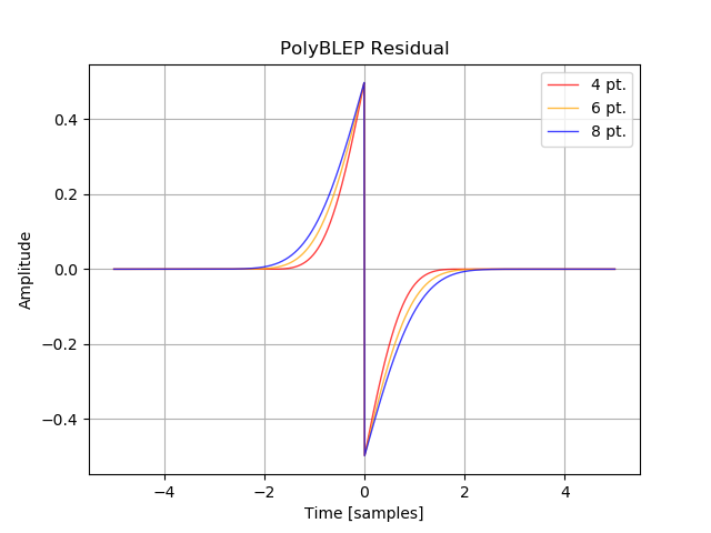
JB_8_7(t) := t^8/40320;PolyBLEP residual をプロットします。コードを実行すると 4 point PolyBLEP residual をプロットします。 6 point と 8 point を含む完全な実装は次のリンク先に掲載しています。
import numpy as np
import matplotlib.pyplot as plt

def polyBlep4(t):
    if t < -2:
        return 0
    if t < -1:
        t += 2
        return t**4 / 24
    if t < 0:
        t += 1
        return -t**4 / 8 + t**3 / 6 + t**2 / 4 + t / 6 + 1 / 24
    if t < 1:
        return t**4 / 8 - t**3 / 3 + (2 * t) / 3 - 1 / 2
    if t < 2:
        t -= 1
        return -t**4 / 24 + t**3 / 6 - t**2 / 4 + t / 6 - 1 / 24
    return 0

def polyBlepResidual(time, basisFunc):
    return np.array([basisFunc(t) for t in time])

nSample = 5

time = np.linspace(-nSample, nSample, 1024)

residual4 = polyBlepResidual(time, polyBlep4)

plt.title("PolyBLEP Residual")
plt.plot(time, residual4, lw=1, alpha=0.75, color="red", label="4 pt.")
plt.xlabel("Time [samples]")
plt.ylabel("Amplitude")
plt.legend()
plt.grid()
plt.show()
出力されたプロットです。論文の Fig. 1. (c) と似たような形になりました。
PolyBLEP residual を入力信号と足し合わせるときにパラメータの向きについて混乱したので図にしました。

\(J B_{i,j}\) の \(i\) は PolyBLEP residual の点数、 \(j\) は PolyBLEP residual を足し合わせるサンプルの位置を表しています。
\(t\) は時間の進む方向と逆行します。
正しく動作するかを確認するために、矩形波に PolyBLEP residual を足し合わせて周波数特性を出します。
長いので 4 point の実装だけを掲載します。この実装は PolyBLEP の点数と同じサンプル数だけ出力が遅れます。次のリンクは 6 point と 8 point の実装を含んだコードです。
import numpy as np
import matplotlib.pyplot as plt
import scipy.signal as signal
class SquareOscillator:
def __init__(self, samplerate, frequnecy):
self.x0 = 0
self.x1 = 0
self.x2 = 0
self.x3 = 0
# 矩形波の high と low が変更された時点を検知する信号。
self.p0 = 0
self.p1 = 0
# g_(n/2) が 0 でないときに PolyBLEP residual の加算をトリガ。
self.g0 = 0
self.g1 = 0
# 分数ディレイ時間。
self.t0 = 0
self.t1 = 0
# 位相の範囲は [0, 2] 。
self.phase = 0
self.tick = 2 * frequnecy / samplerate
def polyBlep4_0(self, t):
return -t**4 / 24 + t**3 / 6 - t**2 / 4 + t / 6 - 1 / 24
def polyBlep4_1(self, t):
return t**4 / 8 - t**3 / 3 + (2 * t) / 3 - 1 / 2
def polyBlep4_2(self, t):
return -t**4 / 8 + t**3 / 6 + t**2 / 4 + t / 6 + 1 / 24
def polyBlep4_3(self, t):
return t**4 / 24
def process4(self):
self.p1 = self.p0
self.p0 = 1 if self.phase < 1 else -1
self.x3 = self.x2
self.x2 = self.x1
self.x1 = self.x0
self.x0 = self.p0
self.g1 = self.g0
self.t1 = self.t0
if self.p0 == self.p1:
self.g0 = 0
self.t0 = 0
else:
self.g0 = self.x0 - self.x1
self.t0 = (self.phase - np.floor(self.phase)) / self.tick
if self.g1 != 0:
t = max(0, min(self.t1, 1)) # 念のため。
self.x0 += self.g1 * self.polyBlep4_0(t)
self.x1 += self.g1 * self.polyBlep4_1(t)
self.x2 += self.g1 * self.polyBlep4_2(t)
self.x3 += self.g1 * self.polyBlep4_3(t)
self.phase += self.tick
if self.phase >= 2:
self.phase -= 2
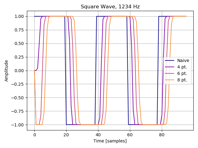
return self.x3出力波形です。 PolyBLEP residual
を足し合わせた波形は角が鈍っています。 Naive は scipy.signal.square
の波形です。
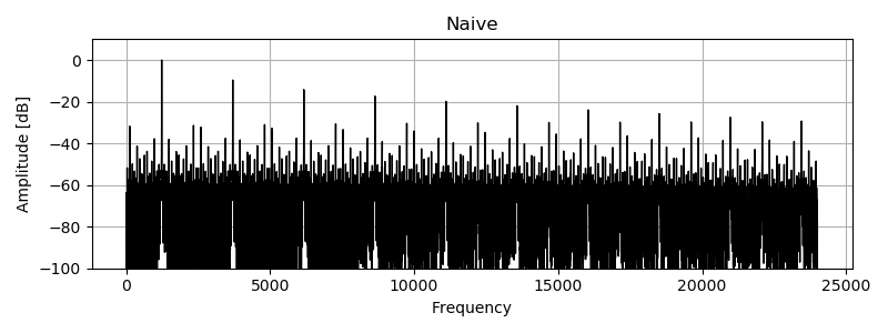
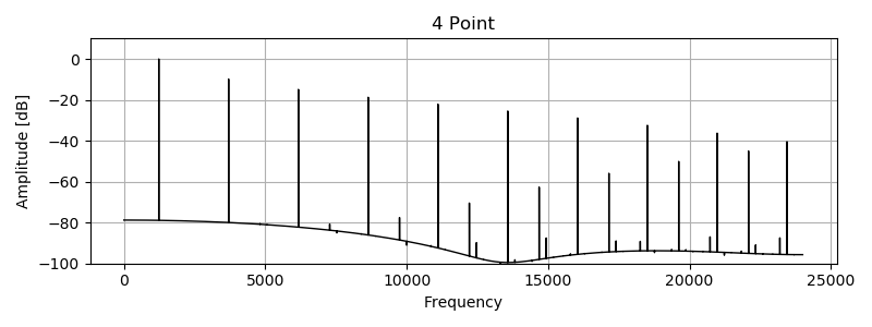
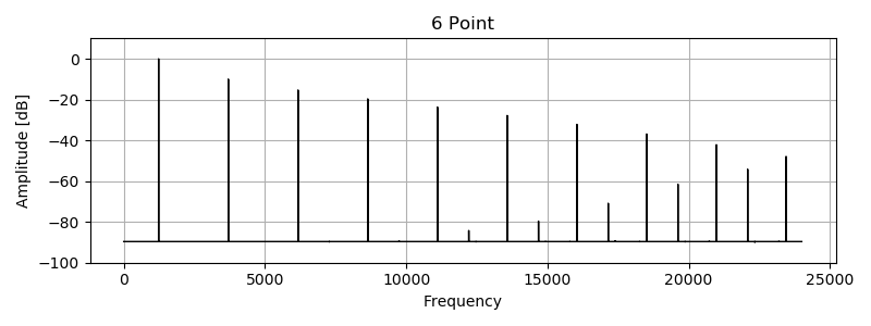
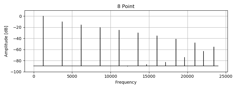
パワースペクトラムです。矩形波の周波数は 1234 Hz 、プロットに使ったサンプリング周波数は 48000 Hz です。 PolyBLEP residual によってエイリアシングノイズが低減されています。
Nam, J., Pekonen, J., & Valimaki, V. (2011). Perceptually informed synthesis of bandlimited classical waveforms using integrated polynomial interpolation.
SquareOscillator の t0
が間違っていたので修正。