何かあれば GitHub のリポジトリに issue を作るか ryukau@gmail.com までお気軽にどうぞ。
Update: 2025-01-07
Golly の Genrations というセルオートマトンのルールを使って音を作りました。
似たような音に分類したくなったので、音のMFCCを特徴としてK-Meansでクラスタリングしました。
Golly の generations から生成した音のデータセットを次のリンクからダウンロードできます。
7zipで解凍できます。
$ 7z x golly_generations_cluster.7z解凍してできる cluster 内の generations
がデータセットです。その他のディレクトリはクラスタリングの結果です。
手始めに次のようなコードを書きました。
scipy.signal.spectrogram から得たスペクトログラムを
numpy.ravel で1次元にして
sklearn.cluster.KMeans でクラスタリングしています。
計算に時間がかかるので numpy.save
で計算結果を保存しています。
import numpy
import scipy.signal
import sklearn.cluster
import shutil
import soundfile
from pathlib import Path

def extract_feature(path, n_frame=39):
    """
    スペクトログラムは2次元のデータ。
    sklearn.cluster で使えるように numpy.ravel で1次元にして返す。

    spectrogram.shape = (n_freq, n_frame)

    n_frame のデフォルト値はテストに使ったデータセットを調べて決めた。
    """
    data, samplerate = soundfile.read(str(path))
    frequency, time, spectrogram = scipy.signal.spectrogram(data, samplerate)

    if spectrogram.shape[1] < n_frame:
        zeros = numpy.zeros((spectrogram.shape[0],
                             n_frame - spectrogram.shape[1]))
        spectrogram = numpy.concatenate((spectrogram, zeros), axis=1)
    elif spectrogram.shape[1] > n_frame:
        spectrogram = spectrogram[:][0:n_frame]

    return numpy.ravel(numpy.transpose(spectrogram))

def write_result(output_directory, n_clusters, labels, filepath):
    if output_directory.exists():
        shutil.rmtree(output_directory)

    digits = len(str(abs(n_clusters - 1)))
    output_directories = [
        output_directory / Path(f"{index:0{digits}d}")
        for index in range(n_clusters)
    ]

    for directory in output_directories:
        directory.mkdir(parents=True, exist_ok=True)

    for label, path in zip(labels, filepath):
        shutil.copy(path, output_directories[label])

if __name__ == "__main__":
    directory_path = Path("generations")
    if not directory_path.is_dir():
        print("Invalid path.")

    filepath = [path for path in directory_path.glob("*.wav")]
    features = numpy.array([extract_feature(path) for path in filepath])

    n_clusters = 40
    cluster = sklearn.cluster.KMeans(n_clusters=n_clusters).fit(features)

    write_result(
        Path("cluster_spectrogram"), n_clusters, cluster.labels_, filepath)

    numpy.save("data/filepath.npy", filepath)
    numpy.save("data/features.npy", features)
    numpy.save("data/features_shape.npy", (39, 129))
    numpy.save("data/labels.npy", cluster.labels_)
numpy.save("data/centers.npy", cluster.cluster_centers_)耳で聞いた印象がいまいちだったので sklearn.cluster
の中から次のクラスタリング手法を試しました。
KMeansAffinityPropagationAgglomerativeClusteringSpectralClusteringDBSCANAgglomerative と KMeans
は似たような結果が出ました。
AffinityPropagation
はアルゴリズム側でクラスタの数を自動的に決めてくれます。
damping
をデフォルトの0.5にするとクラスタの数が多くなりすぎたので、適当に0.6としたところ119のサンプルに対して60ほどあったクラスタが15まで減りました。
SpectralClustering の結果は良くなかったです。
DBSCAN
はサンプルの数と同じだけのクラスタができる結果となりました。Visualizing
DBSCAN Clustering
を見ると空間を格子に区切って、格子内のデータポイントの数に応じてクラスタを作っています。今回のデータでは次元の高さに対してデータポイントの数が少なすぎるためにクラスタが形成されにくいのかもしれません。
ここでは Golly の generations で作った音のクラスタリングには
KMeans で十分と判断しました。
クラスタリング手法では結果が改善しないこともわかったので特徴抽出を変えることにしました。
numpy.spectrogram
を使ったクラスタリングの結果に満足できなかったので python_speech_features
をインストールして MFCC
を使うことにしました。
プロトタイプの extract_feature
を次のように変更しました。
import python_speech_features

def extract_feature(path, n_frame=19):
    """
    mfcc.shape = (n_frame, n_cepstrum)
    """
    data, samplerate = soundfile.read(str(path))
    nfft = 1024
    mfcc = python_speech_features.mfcc(
        data,
        samplerate,
        winlen=nfft / samplerate,
        winstep=0.01,
        numcep=26,
        nfilt=52,
        nfft=nfft,
        preemph=0.97,
        ceplifter=22,
    )

    if mfcc.shape[0] < n_frame:
        zeros = numpy.zeros((n_frame - mfcc.shape[0], mfcc.shape[1]))
        mfcc = numpy.concatenate((mfcc, zeros), axis=0)
    elif mfcc.shape[0] > n_frame:
        mfcc = mfcc[0:n_frame]

    return numpy.ravel(mfcc)
winlen * samplerate > nfft のときにエラーが出るので
winlen は nfft の値から決めています。
numcep と nfilt
は適当にデフォルトの2倍にしました。
Golly の generations
で作った音は低周波成分がそれなりに含まれるので、ルールと音の関係を調べるなら
preemph
は0でいいかもしれません。ここでは耳での聞こえ方で分類したかったのでデフォルト値を使っています。
Golly の generations で作った音のクラスタリングについては、MFCCを使うことでスペクトログラムを使うよりも私の主観では良い結果が出ました。データポイントの次元が減るので計算も早くなります。
KMeans のパラメータ n_clusters
を決めるために elbow
method を試しました。
KMeans
の誤差はクラスタの数を増やすと小さくなります。また、クラスタの数が増えると誤差の減り方が緩やかになってきます。
Elbow method
では誤差の減り方が十分に緩やかな範囲で最も小さいクラスタの数を使います。誤差の減り方が緩やかかどうかの判断はデータセットに応じて人間が適当に行うようです。
実装では sklearn.cluster.KMeans.inertia_
がそのまま使えます。
import matplotlib.pyplot as pyplot
import numpy
import python_speech_features
import sklearn.cluster
import soundfile
from pathlib import Path
def get_inertia(n_clusters, features):
cluster = sklearn.cluster.KMeans(n_clusters=n_clusters).fit(features)
return cluster.inertia_
if __name__ == "__main__":
features = numpy.load("features.npy")
x_range = (2, 101)
errors = [get_inertia(k, features) for k in range(*x_range)]
k_value = [k for k in range(*x_range)]
pyplot.plot(k_value, errors, lw=1, color="gray")
pyplot.plot(k_value, errors, "o", markersize=3, color="black")
pyplot.xlabel("n_clusters")
pyplot.ylabel("error")
pyplot.xlim((x_range[0], x_range[1] - 1))
pyplot.grid()
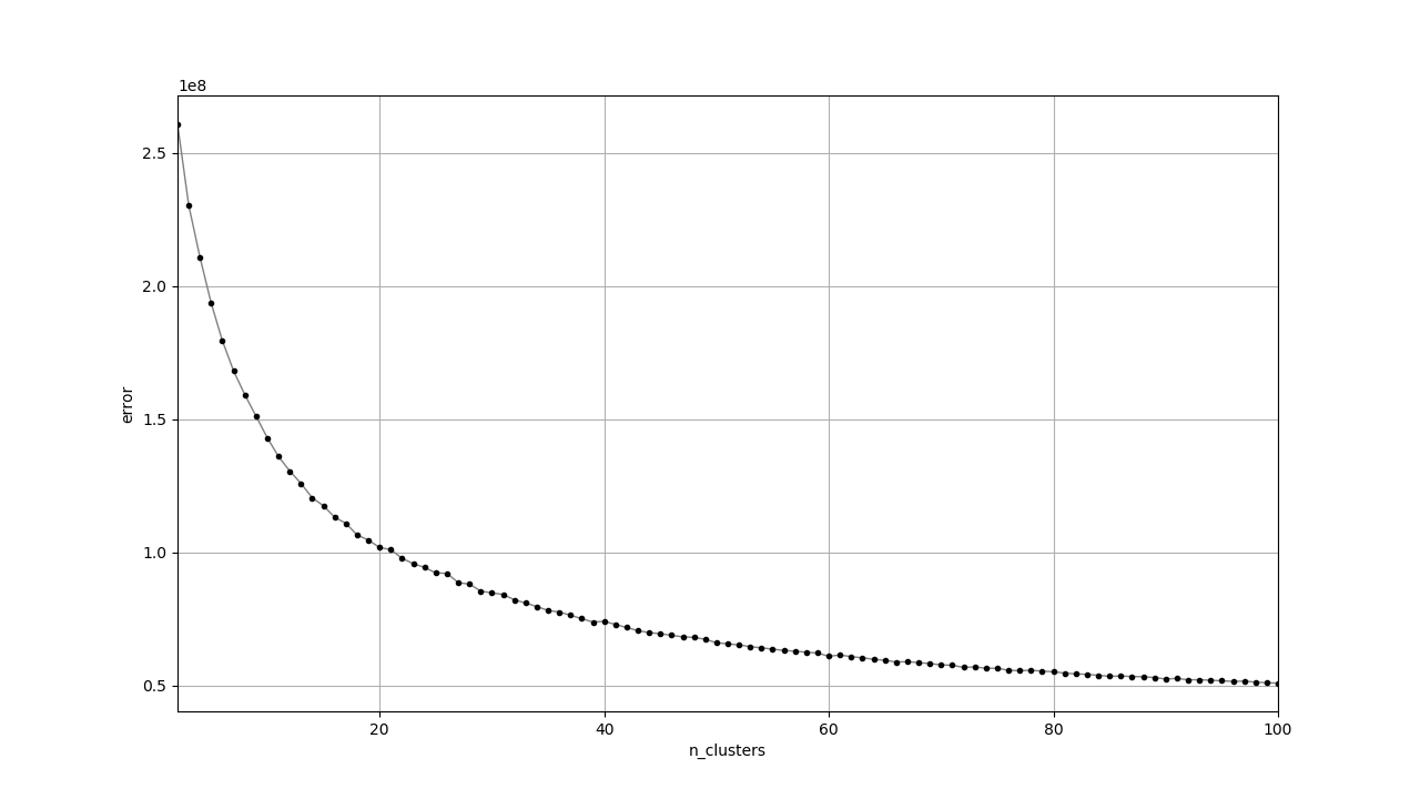
pyplot.show()出力されたプロットです。
滑らかで elbow
となる傾きが急に変わる箇所がないように見えます。今回は特に目的も正解もなくクラスタリングしているので
k=40 くらいでいい気がします。
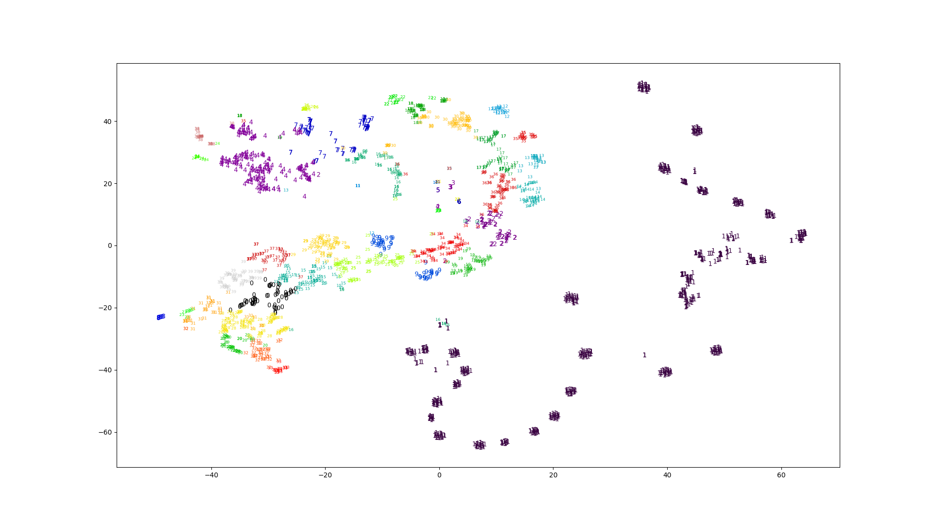
いい評価方法が思いつかないので、とりあえず t-SNE で視覚化しました。
sklearn.manifold.TSNE
を使います。
import numpy
import sklearn.manifold

features = numpy.load("data/features.npy")
tsne = sklearn.manifold.TSNE(n_components=2).fit(features)
numpy.save("data/embedding.npy", tsne.embedding_)
計算結果のプロットです。図の数字はデータポイントの属するクラスタの番号と対応しています。
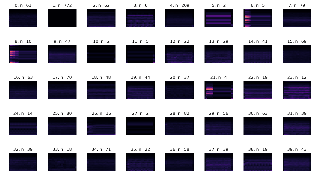
クラスタの内容を調べるために適当に思いついたパラメータをプロットします。
中央値が表すMFCCです。各画像の縦が周波数で下から上に向かって大きくなります。横は時間で左から右に向かって進んでいます。明るい部分ほど係数が大きくなります。
n
はクラスタに含まれるデータポイントの数を表しています。
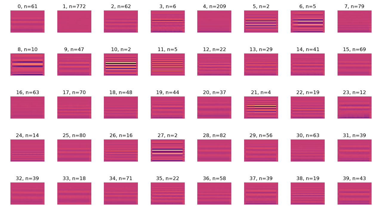
K-Meansの中央値と対応するデータポイントとの間での平均絶対誤差 (mean absolute error) です。
以下は耳で聞いた印象です。
特徴ベクトルを変えて出力したプロットを別ページにまとめました。
ここではクラスタリングの結果について、ざっくり耳で聞いた判断しか行っていません。
MFCCを試した後でスペクトログラムを改善できないか試しました。
numpy.log で対数に変換。どちらもMFCCと比べて良くなったとは感じませんでした。
Elbow method
はヒューリスティックのわりに計算に時間がかかります。今回のような正解となるデータセットがない状態でのクラスタリングでは
KMeans よりも、自動的にクラスタの数を決めてくれる
AffinityPropagation を使ったほうが楽かもしれません。